


Data from Hugging Face and CMU research
BUT, we can take action to reduce thatScroll Down to Learn More
Hi! My name is Alvin Chen. I created this website to share my research on "Reducing Carbon Emissions in AI Image Generation at the Inference Stage."
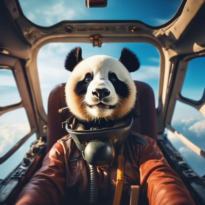
AI image generation is a groundbreaking technology that produces stunning visuals and drives innovation. However, it comes with a hidden cost: its environmental impact. With approximately 34 million AI-generated images created daily, the energy required results in substantial carbon emissions—about 120,000 pounds of CO₂ every day. This is equivalent to about 54 metric tons daily!
While much attention has been given to the energy demands of training AI models, most of the carbon footprint actually occurs during the inference stage—the process of generating images. Surprisingly, this area remains underexplored in research. My goal was to address this gap by evaluating strategies to reduce emissions without sacrificing performance.
In my research, I focused on the following key factors:
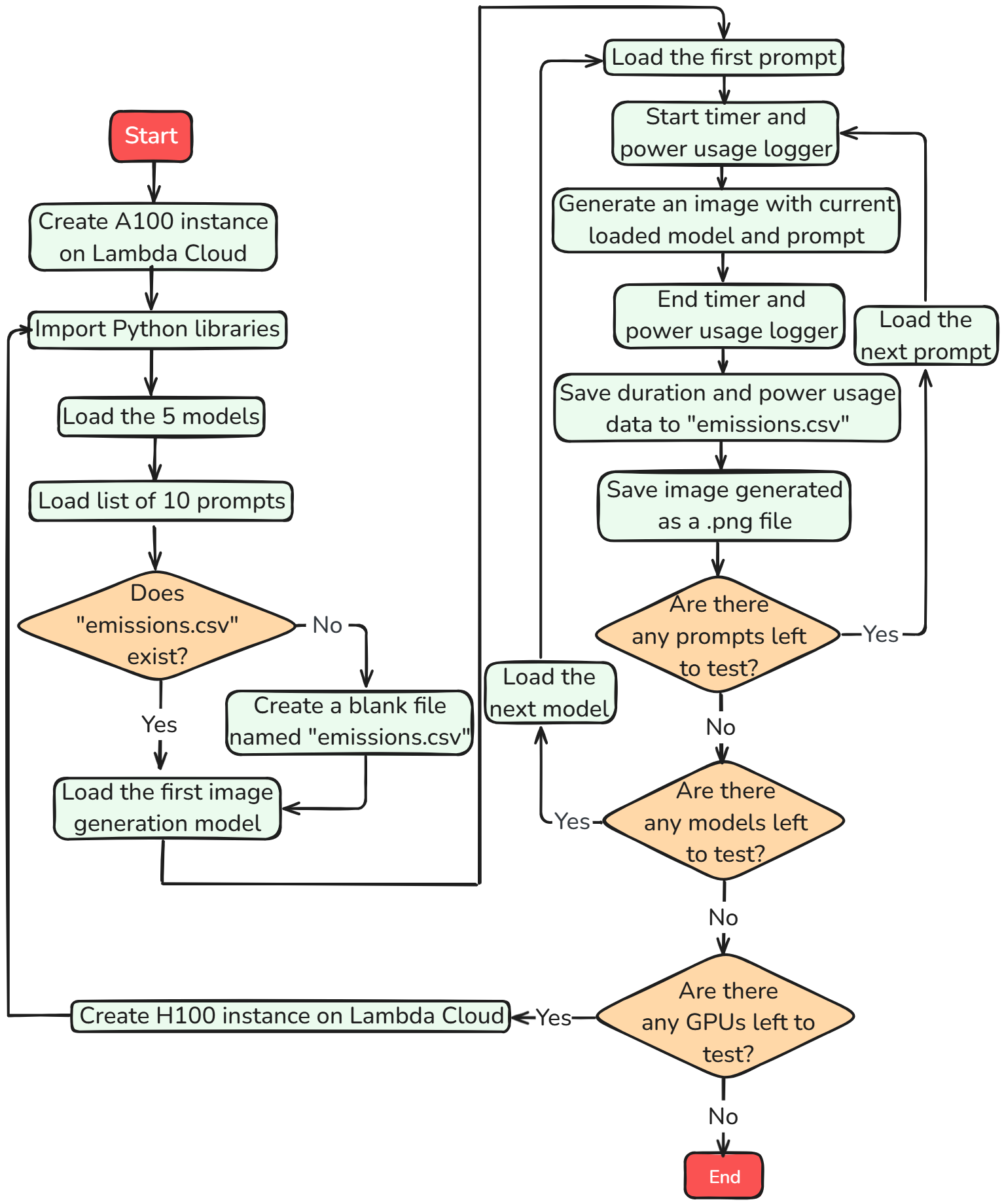
To achieve this, I tested five open-source models, ran simulations with real-world data patterns, and calculated emissions using regional carbon intensity metrics. My findings offer actionable insights for both individuals and companies generating AI images.
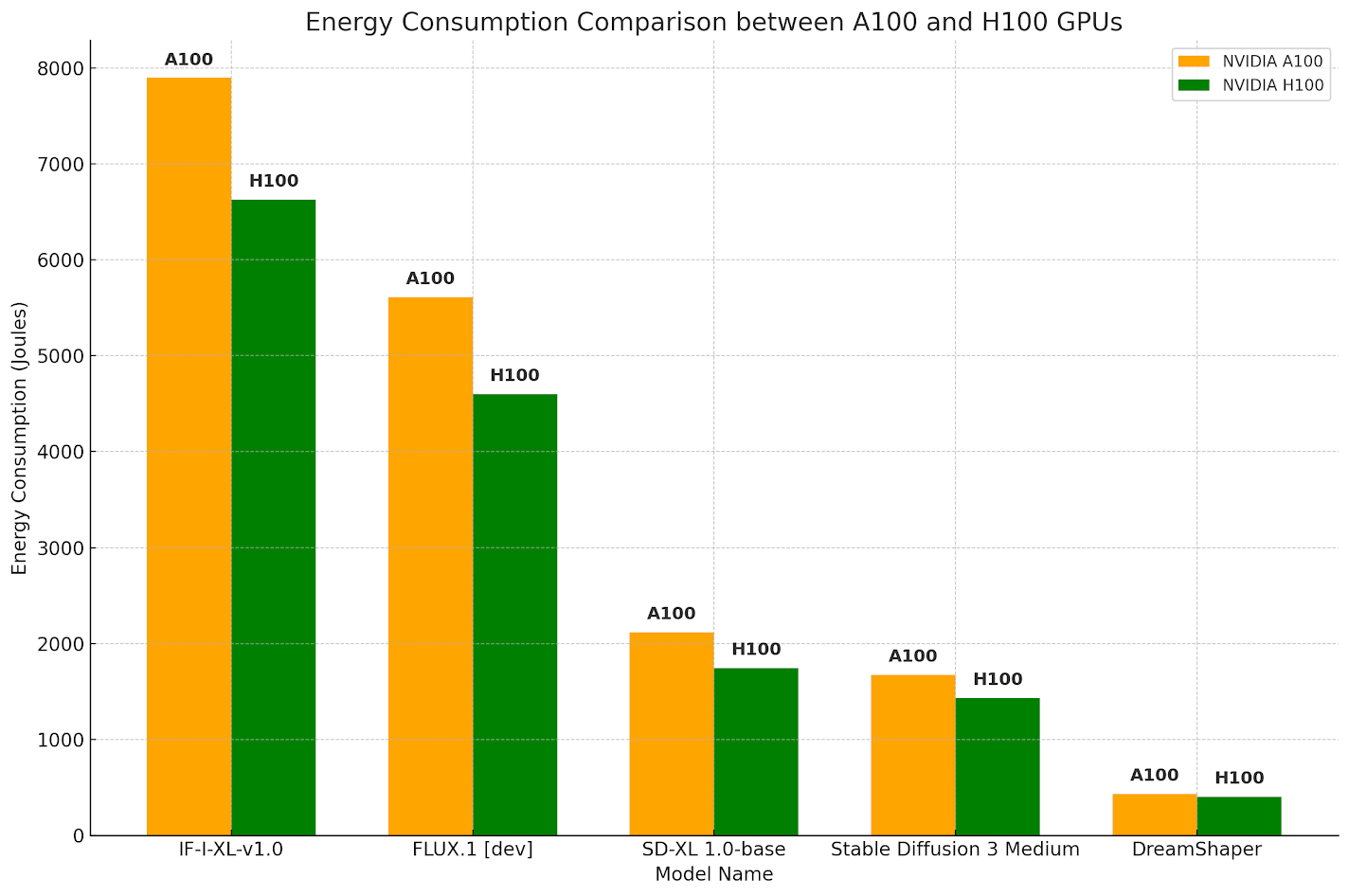
The model used to generate the image affects the number of operations necessary to complete the image generation. Along with the GPU choice, the model choice determines how much energy is consumed during generation.
The GPU used to generate the image affects the speed at which the operations are processed as well as the power usage. Along with the model choice, the GPU choice determines how much energy is consumed during generation.
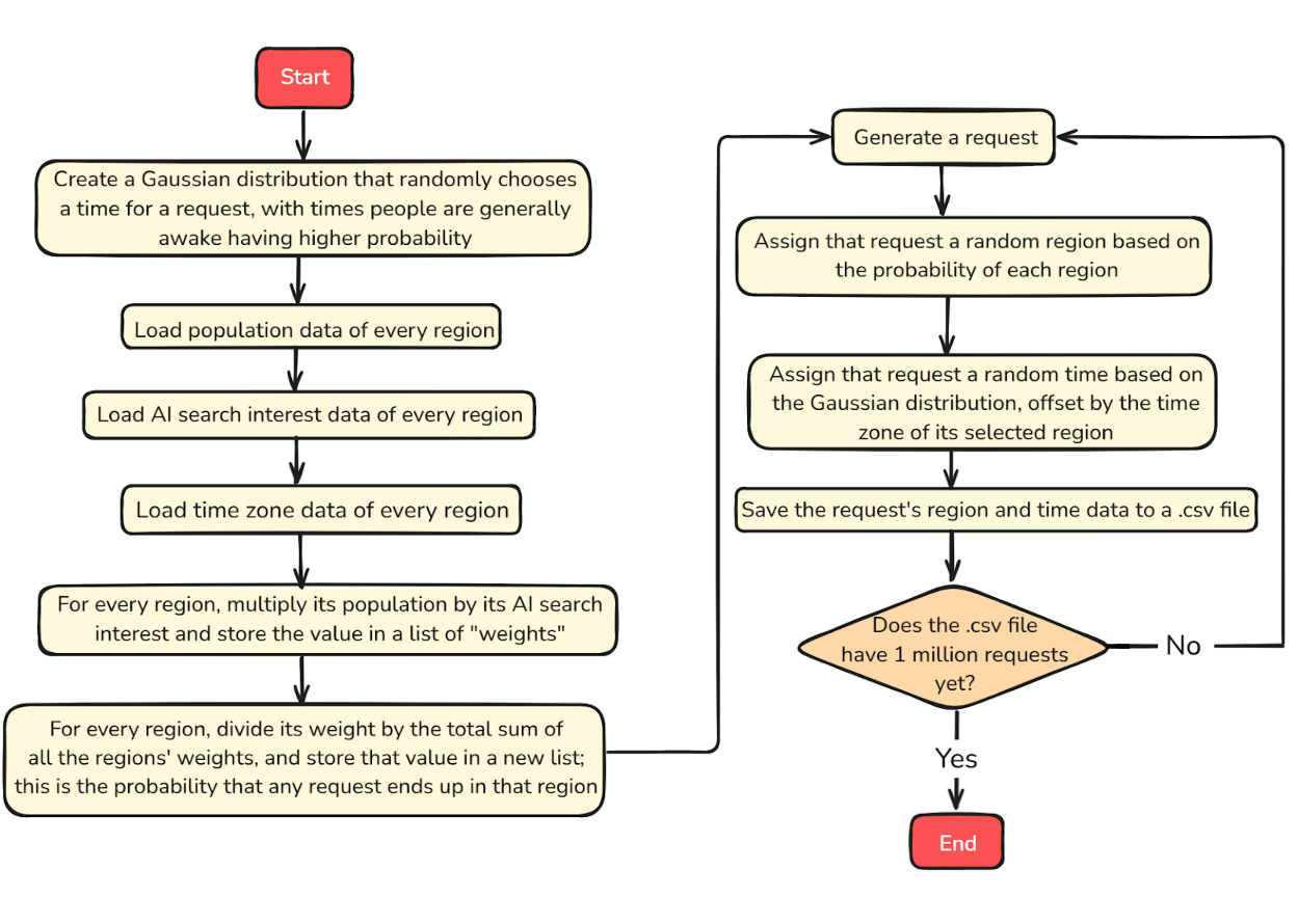
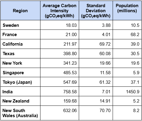
The carbon intensity is defined as the amount of greenouse gas emissions per unit of energy consumed. The location where the image is generated affects the carbon intensity of image generation since some regions have an energy mix containing more clean energy sources than others.
The time when the image is generated also affects the carbon intensity of image generation due to the inherent variability of renewable energy caused by the unpredictability of weather conditions. For example, when it's cloudy, carbon intensity increases since less solar energy would be produced and more fossil fuels would have to be burned.
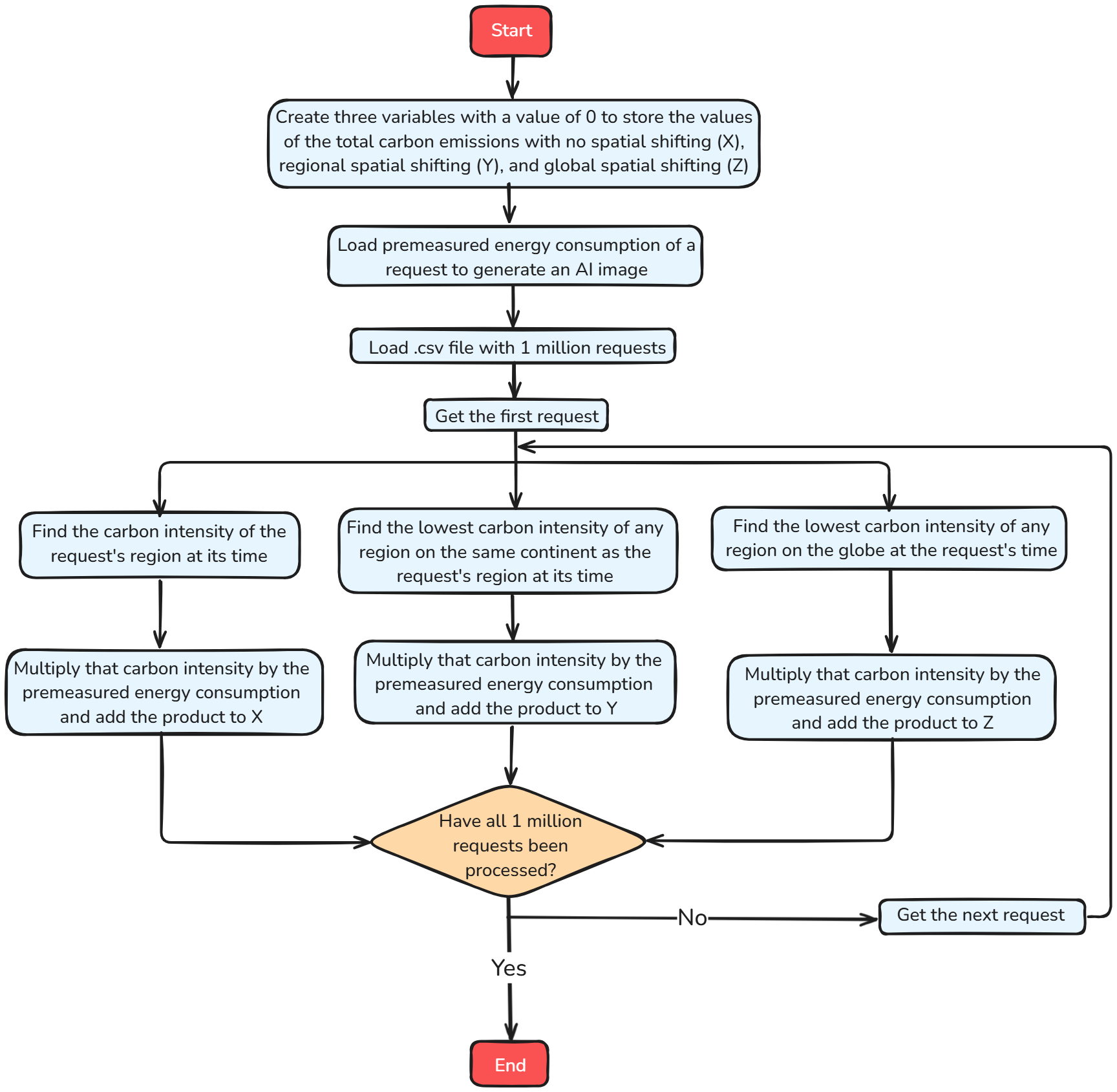
To calculate the carbon emissions from AI image generation, use this formula:
Power Consumption x Time x Carbon IntensityImage Scoring Criteria:
1 - Unacceptable
2 - Needs improvement
3 - Acceptable
4 - Good quality
5 - Accurate to the prompt, high quality
Prompt 1:
A bustling medieval marketplace with people in period clothing, merchants selling goods from wooden stalls, and a castle looming in the background.
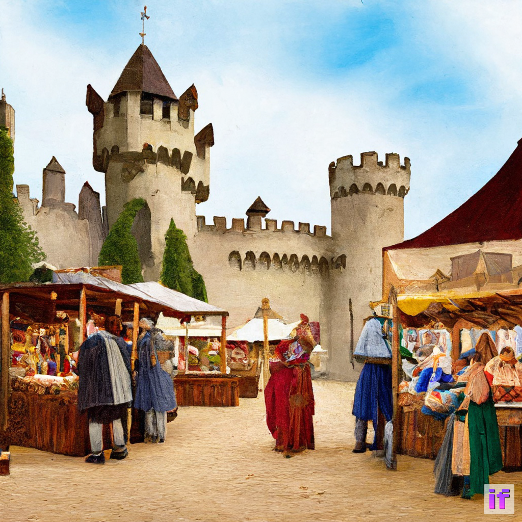
Score: 3
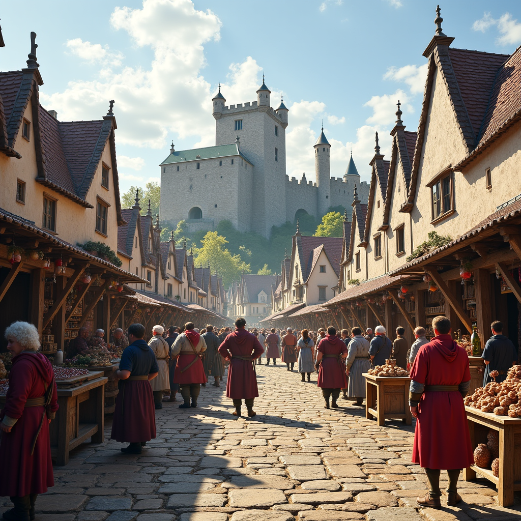
Score: 5
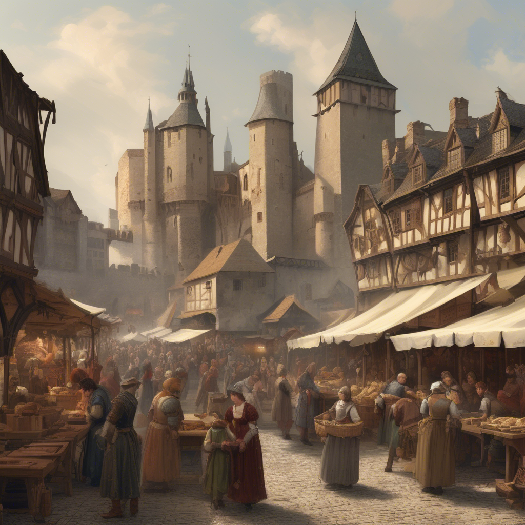
Score: 4
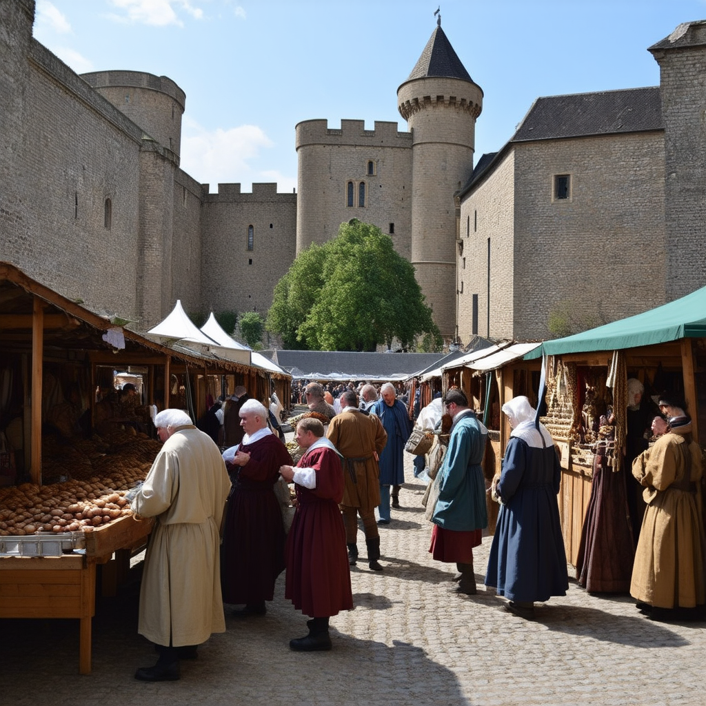
Score: 5

Score: 4
Prompt 2:
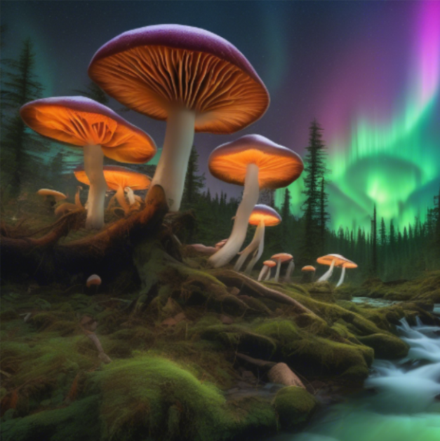
A mystical forest with glowing mushrooms, towering ancient trees, and a crystal-clear stream running through it. The sky is filled with vibrant auroras.
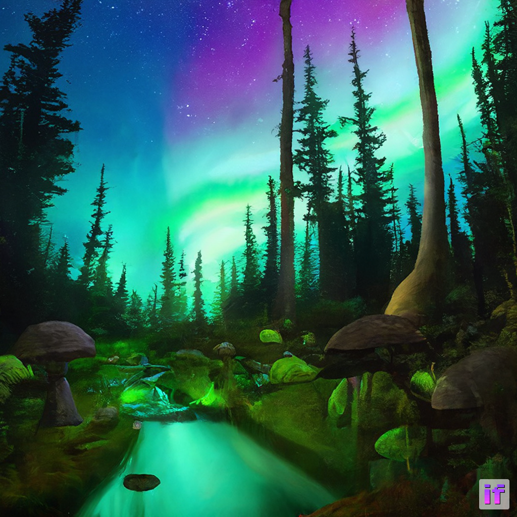
Score: 3
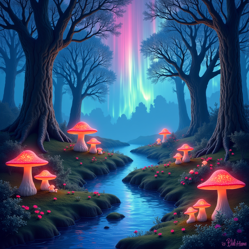
Score: 5
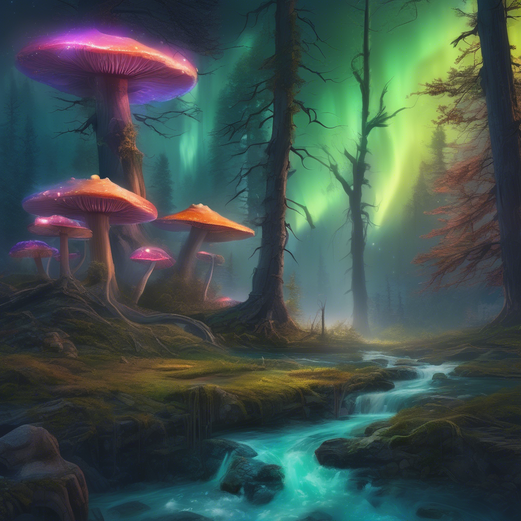
Score: 5
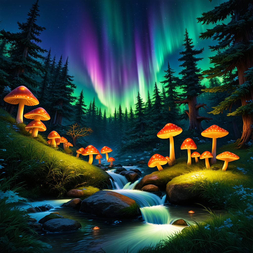
Score: 5
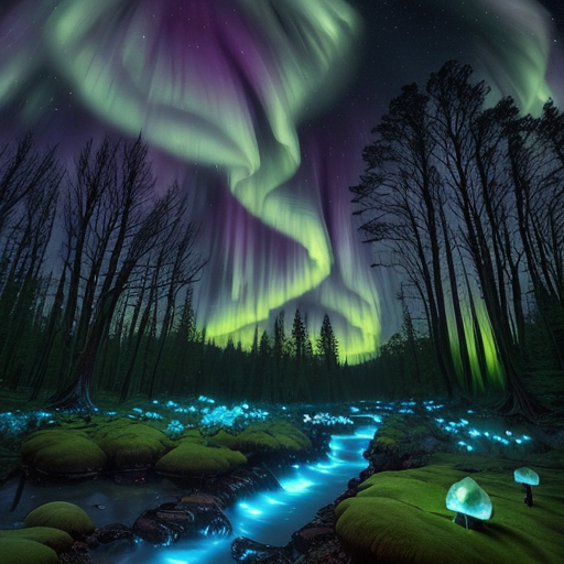
Score: 4
Prompt 3:
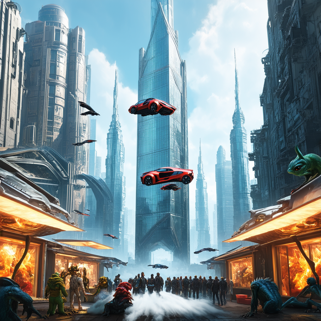
A futuristic city with towering skyscrapers made of glass and metal, flying cars zooming by, and a vibrant, bustling marketplace filled with alien creatures.
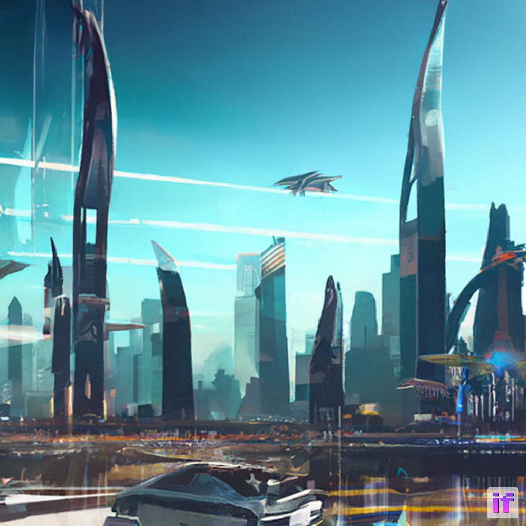
Score: 2
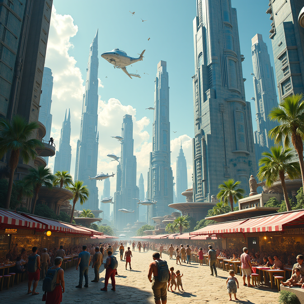
Score: 4
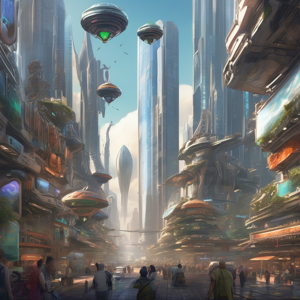
Score: 3
Score: 5
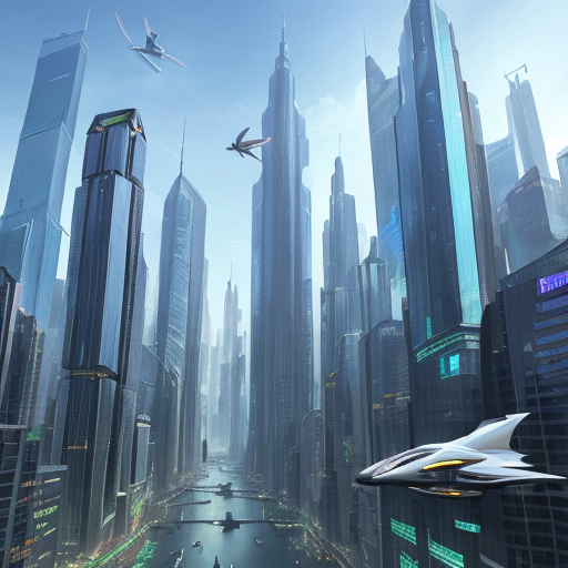
Score: 4
Prompt 4:
A colorful, swirling pattern of geometric shapes and lines, with a focus on bright blues, reds, and yellows, evoking a sense of motion and energy.
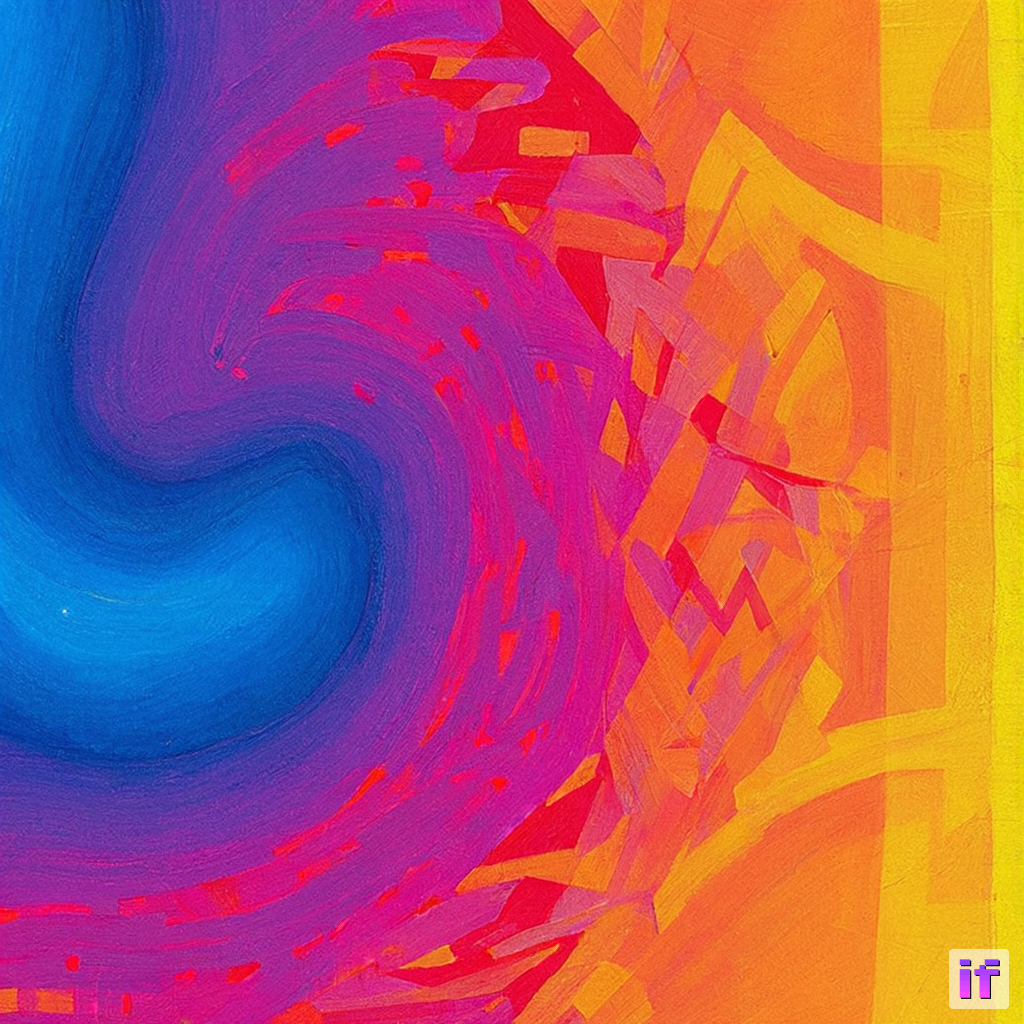
Score: 3
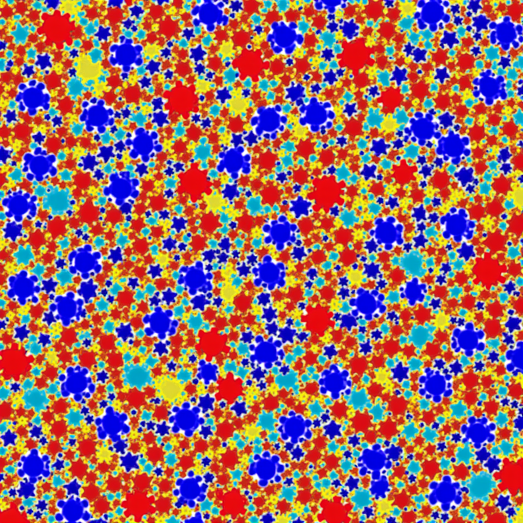
Score: 4

Score: 4

Score: 5
Score: 4
Prompt 5:
A detailed, realistic portrait of a young woman with curly hair, wearing a vintage dress, sitting by a window with soft sunlight illuminating her face.

Score: 4

Score: 5

Score: 4
Score: 5

Score: 5
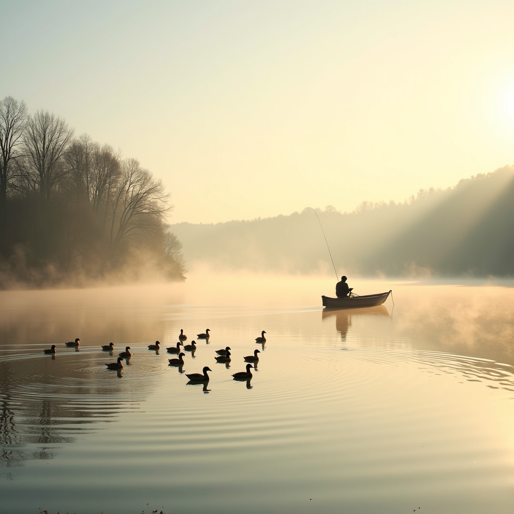
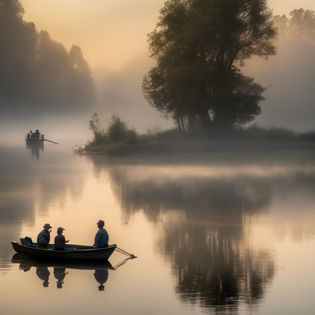
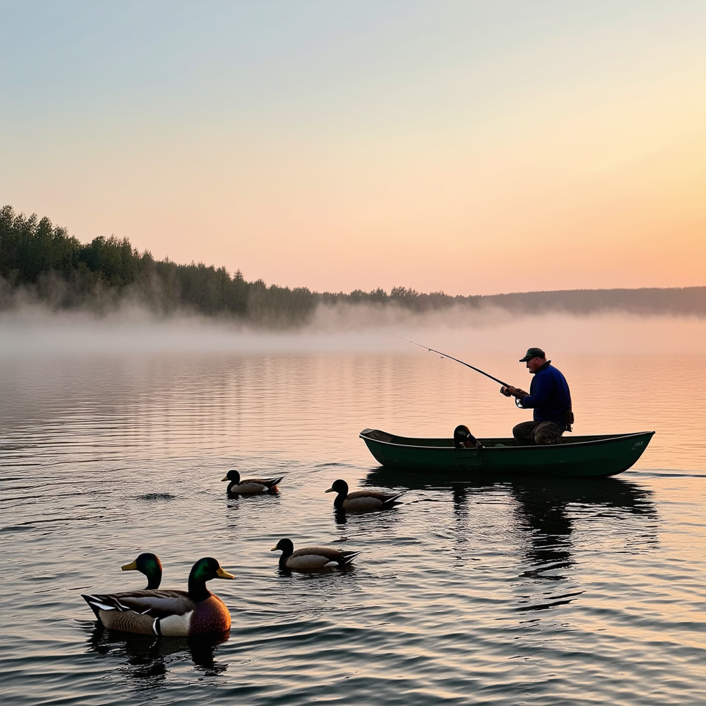
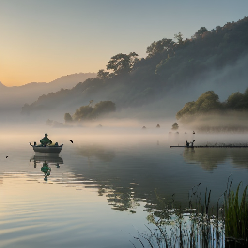
Prompt 6:
A serene lakeside scene at dawn, with mist rising from the water, a family of ducks swimming by, and a fisherman in a small boat casting his line.
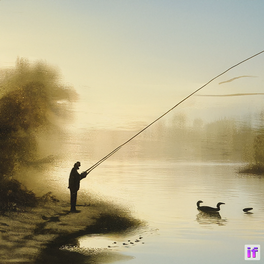
Score: 1
Score: 5
Score: 4
Score: 5
Score: 4
Prompt 7:
A gritty city street with vibrant graffiti covering the walls, a breakdancer performing in the foreground, and bystanders watching and taking pictures.

Score: 2

Score: 5

Score: 3
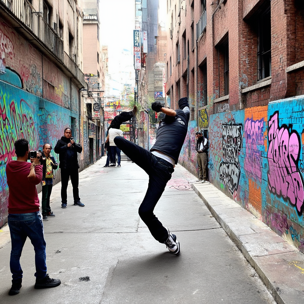
Score: 3

Score: 2
Prompt 8:
A majestic dragon with shimmering scales, large wings, and piercing eyes, perched on a mountain peak with a stormy sky in the background.

Score: 2

Score: 4
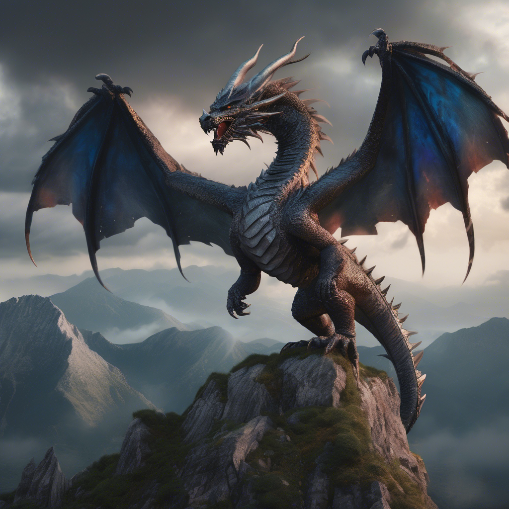
Score: 4

Score: 5
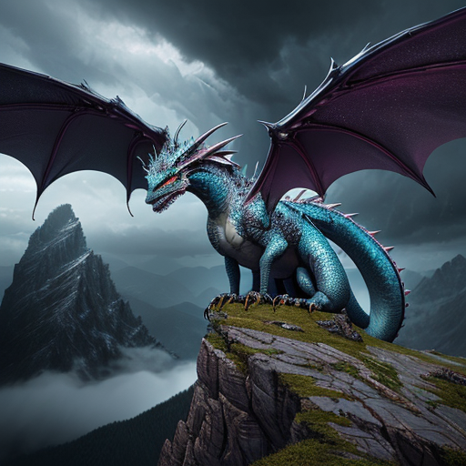
Score: 4
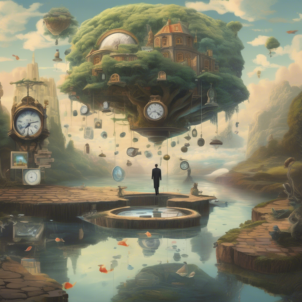
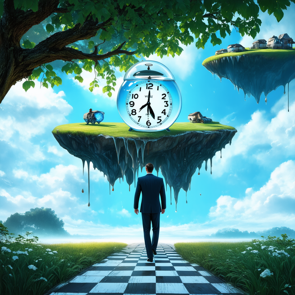
Prompt 9:
A dream-like scene with floating islands, a giant clock melting over a tree branch, and a man in a suit with a fishbowl for a head walking on a checkerboard path.

Score: 1
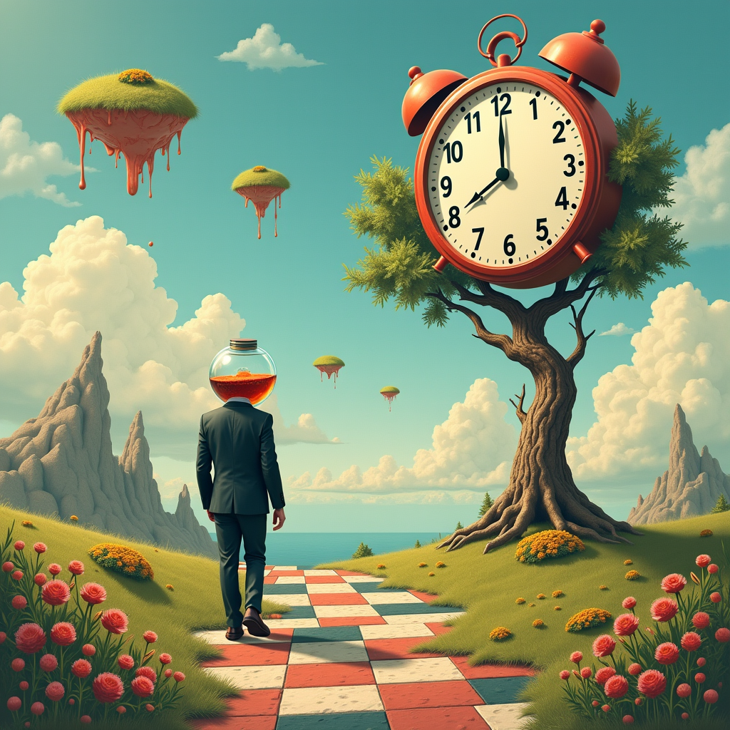
Score: 4
Score: 2
Score: 3
Score: 4
Prompt 10:
A dynamic action scene with a superhero in a colorful costume flying through the air, about to clash with a menacing villain, with bold lines and vibrant colors.

Score: 3

Score: 5

Score: 4

Score: 4
Score: 5
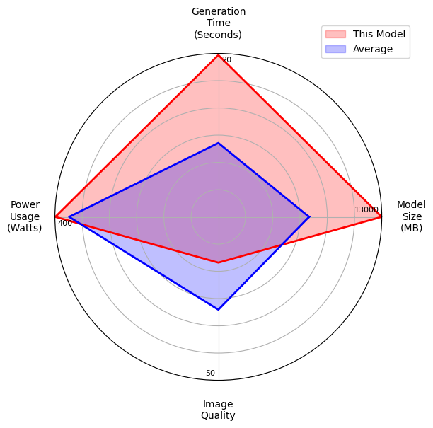
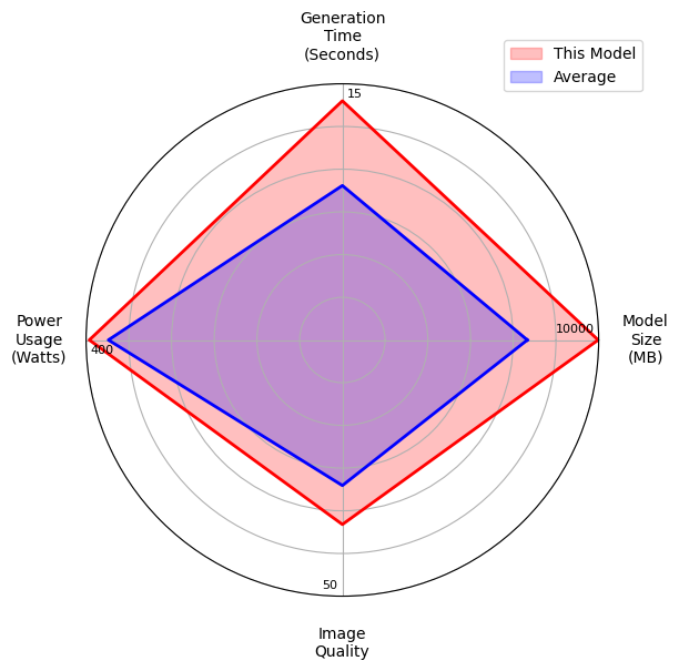
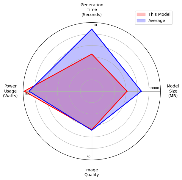
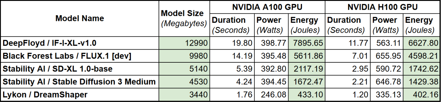
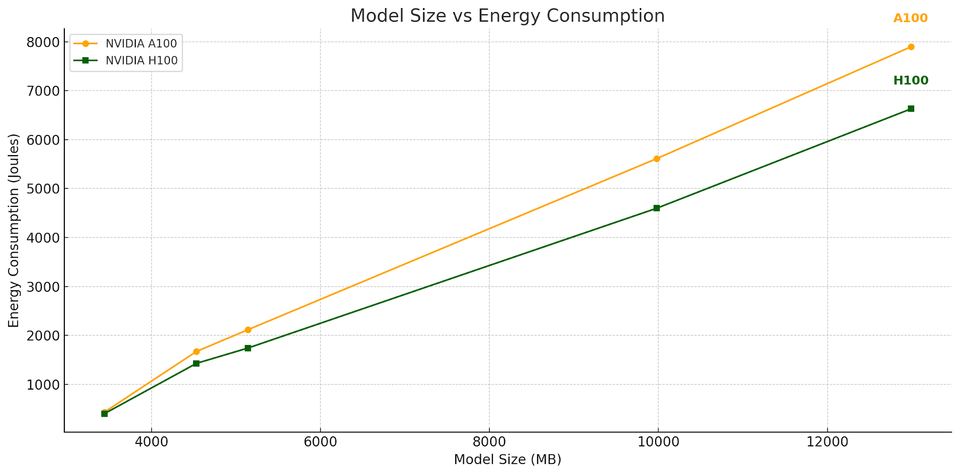
To evaluate the impact of model choice on carbon emissions, let's analyze the properties of these AI image generation models.
 DeepFloyd / IF-I-XL-v1.0
IF-I-XL-v1.0, developed by the AI research lab DeepFloyd, is the largest and most carbon-intensive model among the five. Despite its scale, it generates low quality images and is not recommended for use.
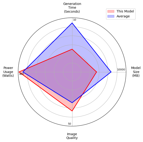
 Black Forest Labs / FLUX.1 [dev]
FLUX.1 [dev], developed by Black Forest Labs, is their most advanced open-source model. While it delivers high quality images, its large model size results in significant emissions and slower response times.
 StabilityAI / SD-XL 1.0-base
SD-XL 1.0-base is one of the latest Stable Diffusion models. With a medium-sized architecture, it delivers good quality images at a reasonable speed. However, it has a high carbon footprint and performs slightly worse than Stable Diffusion 3 Medium across all metrics.
StabilityAI / Stable Diffusion 3 Medium
Stable Diffusion 3 Medium is another one of the latest Stable Diffusion models. It offers high image quality with decent speed, although its carbon emissions remain relatively high.
 Lykon / DreamShaper
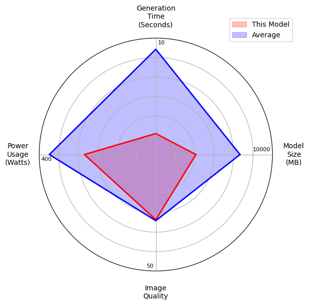
DreamShaper is an improved and fine-tuned version of Stable Diffusion models. As the smallest in model size, it is highly carbon-efficient, producing images quickly with good quality. This model is strongly recommended for all users.
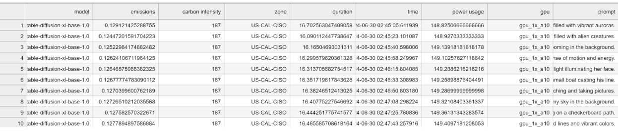
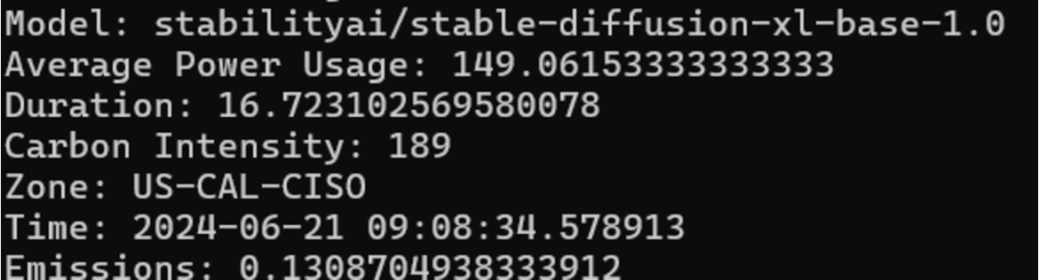
Data Collection and Results Table:


GPUs required = 14 / (5/6) = 16.8


Here are the key observations and findings from my research:
Here are the recommendations based on my research:
Result: grams of CO2